
More than 750 million people use Excel worldwide.
Even a lot of businesses use Microsoft Excel to input and organize various sets of information.
Now you probably know how to input numbers, words and other figures into the rows and columns of an Excel spreadsheet.
But you are probably not utilizing the software to its full potential.
Here are some excel sheet tips and tricks that can help you to use excel spreadsheets like a pro.
How Can You Use Excel or Google Sheet for Business
Can you tell your marketing efforts are successful or profitable without crunching any numbers?
You can’t. And if you don’t properly analyze your marketing data, it’s going to cost your business.
This is why you need to use tools like Excel or Google sheets when you have a large number of figures to add up or analyze.
But before we move ahead to learn some extraordinary formulas for excel cheat sheet, let’s begin with the basics.
First and foremost, you need to get all your information organized in an Excel spreadsheet. Know what’s the source of your data?
Whether it is from your marketing campaigns like email marketing campaigns, SMS campaigns etc. If your data is on some other platform, you need to get those numbers on an excel spreadsheet.
But how do you do it? Manually? It could take hours, weeks, or even months, depending on how much data you have.
A whopping 89 percent of employees admit this data entry as wasting time at work. So here’s your first excel tip.
1. Import Your Data
You can easily import data to an Excel spreadsheet and save your time. To do this, select the “File” menu in a new Excel spreadsheet.
You will find it on the top left corner of your screen. Then select “Import” from the drop-down menu. Click Import, then select your file type on the new box that appears.
Your data is probably in a CSV or HTML file format depending on the platform or lead management system software you’re using.
Once imported, get all your data organized before working on them.
Excel Sheets for Lead Management
Leads are the lifeblood for Sales and salespeople work hard to generate and gather data on their leads.
However, according to Hubspot State of Inbound ’16, 22% of salespeople still don’t know what CRM is, and 40% still use excel sheets and email programs to store customer data.
And one of the reasons they prefer Excel is because they are protective of sharing their contacts with other team members.
This issue can be easily resolved with an integrated sales and marketing tool like Teleduce helps salespeople manage their relationships with leads and customers more effectively.
Along with security, you also get an automated lead scoring process which gives you intelligent insights into the leads.
However, if you still insist on using excel, here are the two functions that will help make your lead management using excel seamless.
Keep reading to know how to manage leads with an excel sheet:
2. VLOOKUP function
What if you had your lead’s name next to their email addresses in one spreadsheet and the same lead’s email addresses with their company names on the other sheet?
How would you get all the data to appear in one place so you can use it wisely for email marketing?
This is where VLOOKUP will come in handy. However, to use this formula, make sure you have once column which is identical in both sheets. Once done, your formula is:
VLOOKUP(lookup value, table array, column number, [range lookup])
Lookup Value: This is the value which is identical in both spreadsheets. If you want to bring data into first spreadsheets, choose the first value in your first spreadsheet.
Table Array: As per the above example, suppose your email column is common and both sheet 1 and sheet 2 and you want to pull data from sheet 2. So, your table array will be “Sheet2!A:B”, where A means Column A in Sheet 2 (which has email) and B means Column B that you want to translate to Sheet 1.
Column Number: The range of column number you enter indicated excel in which column the new data you want to copy to Sheet 1 is located in.
Range Lookup: To make sure you pull in only exact value matches, use FALSE here.
3. Delimited or Fixed Width
What if you want to split up text information between columns?
For example, you want to separate someone’s full name into a first and last name for your email marketing templates, then you can do this with this excel cheat sheet.
Now, “Delimited” in excel means to break up the column based on characters like commas, spaces, or tabs, and “Fixed Width” in excel means to select the exact location on all the columns of the spreadsheet where you want the split to occur.
To do this, highlight the column that you want to split up. Then go to the Data tab and select “Text to Columns.”
You will see a module wherein you select delimited ( to separate full name), then choose your delimiters like a semi-colon, comma, space.
Once you choose it, you can see a preview of what your new columns will look like. If it’s good enough for you, click ‘Next’.
You will then be prompted with Advanced formats if you choose to. When you are done, click “Finish.”
Excel Shortcuts for Data Analysis
With the increased availability of information, the demand for effective data analysis is important to stay competitive for any business.
You can also use Excel to analyze and organize data from your marketing efforts.
And with the rise of social media marketing and analytics, Startups and SMEs now use data analysis to help gain a greater understanding of their audience.
This will also help them make strategic marketing decisions by understanding patterns so that they can make relatively risk-free decisions.
Here’s how you can do it.

4. Trendlines
Chart feature in Excel is invaluable for presenting data for a report or presentation.
But did you know that you use trendlines to predict future values from a given chart?
It is pretty easy to use, just create a chart with your existing data then simply right-click on the plotted line, and select “Add Trendline” from the context menu.
Now you can see that the data represents overall growth.
To the right, you can see a trendline menu with a variety of options that includes different methods of calculating the trend, and even the ability to add a forecast for future months.
5. Pivot Table
To gauge the effectiveness of your marketing campaign, you need to analyze big data.
However, it is tough to analyze large data sets without the help of visual aids.
This is where the Pivot table can make your life easier. You can use them to Summarize, Analyze, Explore and Present data, which are all significant elements in your marketing efforts.
Pivot tables are pretty simple to use and you can find them under the Insert tab.
Here, you will be able to see both the Pivot Tables tool and Recommended Pivot Tables, wherein you can find the most relevant options according to the type of data in your spreadsheet.
To use them, just highlight your data and click on Pivot Tables. You can see a wizard guide with an easy-to-use interface.
Now just click and drag the relevant fields in your data to be used as rows, columns, or filters in the pivot table, and transform your hard-to-digest data into an interactive and easy-to-understand table.
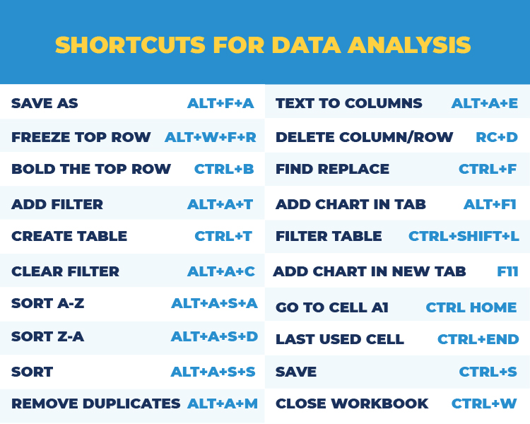
If you use excel of data analysis a lot, then these excel shortcut keys will help you glide through your work much faster.
Begin with saving the file with a name (don’t keep the generic Book1 or whatever name it has) and then prepare it with the following shortcuts which will make it so much easier to work with.
1. Save As: Alt-F-A
2. Freeze Top Row: Alt-W-F-R
3. Bold: Ctrl+B (Bold the top row)
4. Add Filters: Alt-A-T
5. Create Table: Ctrl+T (or Ctrl+L)
Now, once the prep work is done start working with the data, here are some excel shortcuts for data analysis which could prove to be arrows in your quiver.
6. Clear Filter: Alt-A-C
7. Sort A-Z: Alt-A-S-A ( Here “A” is for Ascending)
8. Sort Z-A: Alt-A-S-D (Here “D” is for Descending)
9. Sort Alt-A-S-S: (Here “S” is for Sort)
10. Remove Duplicates: Alt-A-M
11. Text-To-Columns: Alt-A-E
12. Delete Columns/Rows: RC-D (RC means Right click and do this after selecting column/row)
13. Find/Replace: Ctrl+F, . If you need to remove some recurring strings of data, then first enter Find string, then Alt-P, enter Replace value, then Alt-A to replace all
14. Add Chart To the Same Tab: Alt-F1 ( Creates a chart based on the selected data set.)
15. Ctrl+Shift+L: Activate auto filter to data table
16. Add Chart To New Tab: F11
17. Ctrl + Home: Navigates to cell A1
18. Ctrl + End: Navigates to the last cell that contains data
19. Save: Ctrl+S
20. Close Workbook: Ctrl+W
Pro-tip: Check out our guide on Facebook marketing strategy and learn how you can effectively fulfill your marketing goals and collect data from insights to analyze it.
Excel Sheet for Accounting
When it comes to accounting, you probably use excel spreadsheets for analyzing a variety of financial data, from expenditure and income to wages.
These handy excel shortcuts tips will make working with any account a smooth process.
6. Highlighting Data
You probably have a lot of data on a spreadsheet, then to sort it out you certainly need the ability to circle invalid data.
For example, suppose you have an excel sheet on employees’ wages, and you want to find out employees whose salary is below a certain amount.
To find this, first, highlight the data and, from the tabs at the top, go to Data > Data validation. Now choose Data validation again.
You will see a settings tab, where you need to set certain criteria like choose a decimal point. In the Data field, choose “greater than”, and in the Minimum field, enter the amount.
Now again go to the Data validation menu item, and select Circle Invalid Data from the drop-down.
This will circle any cells with a value less than the amount specified.
7. Linking Cells
With linking cells, if you change certain information in one spreadsheet, it can automatically update the same information in another spreadsheet.
This will come in handy, say when you have bank account information in one document and you want to make a statement of financial position document.
For example, if you want to link Sheet A (source) to Sheet B (destination), follow the steps given below:
- In Sheet B, click in the cell that will contain the link formula and type an equal sign = (don’t press Enter).
- Go to the source worksheet, click in the cell that contains the source data (you can now see squiggly lines around it), and press Enter.
- Excel returns you to the destination worksheet and the linked data displays
Excel Sheet for Task Management
Whether you are working with a client or other employees in your company, how do you keep track of everything that needs to be done?
With excel you can create a task list which is just a list of what needs to be done, broken into steps.
Now you can find plenty of task management readymade templates online along with excel shortcuts in pdf format. Also, you can change their format using a pdf converter tool to make it more suitable for use.
These can simplify things for you, but if you want to do it yourself, here are the basic tips.
8. Create Drop-Down List
Using data validation to create drop-down lists in some columns will make it easier to enter the tasks.
To create a drop-down, highlight the cells you want the drop-downs to be in.
Next, click the Data menu in the top navigation and press Validation. Here, you’ll see a Data Validation Settings box open.
Find Allow options, then click Lists and then select your Drop-down List. Check the In-Cell dropdown button, then press OK.

9. Total Task Times
With excel, you can even summarize the estimated and actual task times. This will give you a quick overview, while you enter the tasks, or update them with actual times.
Always remember, the time that you enter is in minutes, so your formula sums all the time, then divided by 60
=SUM(tblTasks[Time Est Minutes])/60
Use Integrated CRM Instead of Excel
Excel can be a lifesaver for startups and small business owners who are just getting started and have limited resources.
It is a pretty straightforward tool and it offers solutions for tracking customer data, creating charts and graphs, and using formulas to complete quick calculations.
But, as your business grows it may not be enough. To streamline your day-to-day tasks, keep your information organized, and work more efficiently, consider using an integrated sales and marketing CRM like Teleduce.
You and your team can access it anytime, anywhere. Also, it can be seamlessly integrated with other business applications like calendars, IVR services, etc to streamline your work and save plenty of your time.
Manage your data more efficiently with Teleduce. Book your free demo today!